I’m sorry. If you’re looking for a completely original, ground-breaking blog post, this one won’t be for you.
There are a lot of visualisations of sorting algorithms. And I mean a lot. Ever wondered what a radix sort sounds like? Now you know. Maybe rainbows are more your thing. Here you go. If I still haven’t convinced you, how about performing a quick sort via the medium of Hungarian folk dance? We’ve got that too.
I rest my case.
Clichés are clichés for a reason though. And frankly, with some many examples already out in the world, what’s the harm in one more. This is the purpose of this blog post; to showcase a sorting algorithm visualisation that I came up with when messing around with the animation module of matplotlib. As is the nature of these visualisations, it turns out that my approach is not completely original even though I did come up with it without seeing anything like it before (great minds think alike, hopefully?). None-the-less, I’ve had a lot of fun writing the code for this project and I love the results so I wanted to share it with the world.
I do not plan to go into detail on the code I have used. If you are curious, you can find it here, well-documented. It’s only a few hundred lines to develop the handful of visualisations featured in this post so definitely worth a scan through if your curious about matplotlib.animation or the sorting algorithms featured in this post.
Instead, I aim to focus on the lay-reader, and use the pretty visualisations as an incentive to introduce some ideas about algorithms and sorting. I have only included a small selection of common sorting algorithms due to limitations of the matplotlib.animation module (or perhaps just limitations of my understanding of it) so perhaps I will return at some point with a more detailed dive into the topic. For now, let’s get right into it.
Introduction
Before we get onto the visualisations (don’t worry, we’ll get there soon), I want to explain how my visualisations are produced so we can understand how their behaviour relates to the mechanics of the sorting algorithms we use.
What’s the Deal with Sorting Algorithms
First though, and you can skip this sounds obvious to you, what is a sorting algorithm?
We are going to be looking at lists of numbers. Specifically, we will be looking at lists in which each element is unique. When we are sorting a list, we only care that the elements are in the correct order, not their actual values and so without loss of generality, we can assume that our list contains the elements $0, 1, 2, \ldots, n-1$ where $n$ is the length of our list. A sorted list of length 5 will look like this:
$$[0,1,2,3,4]$$
Whereas an unsorted list may look like this:
$$[3, 1, 2, 0, 4]$$
The purpose of a sorting algorithm is to take us from a list like the latter to the former. An algorithm is simply a series of instructions that we are to follow in order to achieve the desired result of a sorted list.
There are few rules that we have to follow though. The first is that we can only compare two elements of the list at a time. This may seem very limiting but it makes more sense when we remember that we are writing these algorithms for a computer to use and the architecture of computers is generally limited to these sorts of comparisons.
The Visualisation Method
With the essentials under our belt, let’s take a moment to walk through how my visualisation works. Suppose we have a sorted list of length $n$ containing elements $0,1,\ldots,n-1$. We create $n$ points in our plot each of which corresponding to an element of the list. We colour these points by the value of the element they represent and arrange them in a circle with their angle from north determined by their value. We then shuffle the list so that the elements’ orders become all mixed up. Now that the elements are out of order, we change the radius of each point in the visualisation so that they correspond with how far off each element is from its sorted position. If by chance an element is shuffled to the same place is was initially, it will retain its original radius and stay on the edge of the circle. If in the other extreme an element is moved so that is a far away as possible from its original position then it will move to the center of the circle. In all other circumstances, points will move to somewhere in between. The important thing is, their colour and angular position will not be affected; just their radial position.
As we sort the list we keep updating these radii until the list is sorted again and we return to a perfect circle. To add one more layer of subtlety, we treat the list as cyclic when calculating the distance between a point’s current and initial position. For example if the element $0$ is in position $n-1$ (the last spot in the list) we say that’s its distance from its true position is $1$ and so it will be positioned close to the edge of the circle. Enough introductions though, let’s get to an example. First up: the bubble sort.
The Bubble Sort
The bubble sort is perhaps the simplest sorting algorithm to conceptualise. The process goes as follows:
- We move through the list looking at each pair of elements one by one
- If a given pair is in the correct order then we leave them be
- If the order of a given pair is incorrect, we swap them around
- Once we get to the end of the list we go back to the start and repeat the process
- We continue this until we make no swaps in a given pass through the list, in which case the list must be sorted again
Let’s look at a small example to reinforce this explanation. We start with the unsorted list:
$$[2, 1, 3, 0]$$
We look at the first two elements ($2$ and $1$) first. These are in the wrong order so we swap them to get:
$$[1, 2, 3, 0]$$
The next pair is $2$ and $3$ which happen to be in order so we leave them. We then get to the last pair ($3$ and $0$) which are not in order so we swap them to get:
$$[1, 2, 0, 3]$$
This concludes our first pass through the list. We will then repeat this process twice more until the $0$ is in the correct position and the list is sorted.
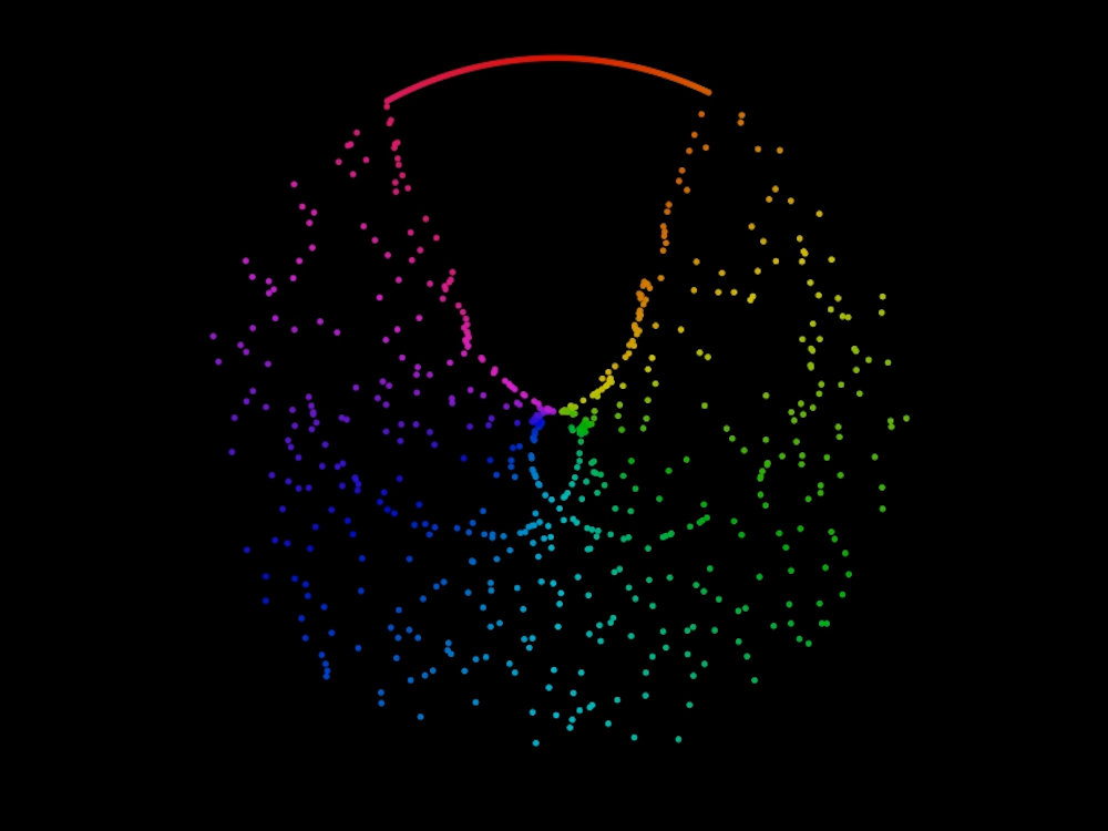
So what does this sorting algorithm look like? Let’s see using a list of length $720$. We start with a sorted list, shuffle it (using Fisher-Yates for those interested) and then proceed to sort it using the bubble sort algorithm. Here is the result:
Wow. Who knew computer science could look so good. We can also spot some interesting characteristics of the bubble sort algorithm. The main observation is that after the $k$th pass through the list, the last $k$ elements are sorted. This is shown in the visualisation by the growing arc starting from the top of the circle and moving anti-clockwise at a uniform rate.Why does the bubble sort elicit this property? Think about it this way: In the first pass through the list, once we have the largest element in the pair we are comparing we will always move it to the right of the other value we are comparing to (if it is not there already). We will then continue to swap it, moving it through the list since, by definition, it is larger than any other element in the list. We now have the largest element fixed in the last position of the list. We then pass through again. We pick up the second largest element in a similar way, carrying it through until we compare it to the largest element, at which point we put it down as in the second largest position. Repeat this for each iteration and the pattern described above develops.
This behaviour of the current largest, unsorted element ‘bubbling’ up to the end of the list is where the algorithm gets its name from.
You may also notice that some points move towards the middle before going back out again. Have a think about why this might be? (Hint: it relates to the cyclic definition of distance we talked about earlier. Suppose the element $0$ gets shuffled to the end of the list; what will its path back be?)
The Selection Sort
We now move on to our second sorting algorithm. This process is very simple to describe although its terrible efficiency means that it is rarely ever used in practice. None-the-less, it may be interesting to visualise.
The algorithm is as follows:
- Pass through the list and note the smallest element
- Move this to the start of the list
- Pass through the list again looking for the second smallest element
- Move this to the second place in the list
- Repeat this process until the list is sorted.
I won’t give an example of this method as it is quite conceptually simple but I would still like to take a moment before we look at the visualisation to ponder what it might look like. Think through the steps described above and imagine what a typical list will look like at the end of each iteration. More importantly, how will this relate to the position of the points in the animation. Hopefully you’ve had a moment of thought so let’s have a look and see whether you were correct.
The Insertion Sort
The next sorting algorithm is one that is likely the most commonly used by humans. It is called the insertion sort. The process goes as follows.
- At each step, suppose that the first $k$ elements are in the correct order (we start with $k=1$ where we only know the first card is in order)
- Take the $(k+1)$th card and insert it into the correct gap between the first $k$ elements (before the first element or after the $k$th are allowed)
- Repeat this process until the list is sorted
This may seem quite confusing but an example will hopefully clear things up. Let’s start with the unsorted list as follows:
$$[3, 0, 1, 2]$$
Vacuously, we know that the first one element(s) is in the correct order. We look at the second element ($0$) and insert it at the start of the list to get
$$[0, 3, 1, 2]$$
We now know that the first two elements are sorted correctly. We look at the third ($1$) and insert it into the first two elements so that their order is correct. That is, we insert it between $0$ and $3$. This gives us:
$$[0, 1, 3, 2]$$
Finally, we know that the first three elements so we look at the fourth ($2$) and insert it between $1$ and $3$ to complete the sorting process.
The corresponding animation for this algorithm looks like this:
Cocktail Sort
Before we close up, we will look at one more sorting algorithm. This is called the cocktail sort. It is a variant of the bubble sort above but rather than always passing through the list in the increasing direction, the algorithm alternates between increasing and decreasing passes. This forwards and backwards motion is the inspiration for the name of this algorithm.
Since this algorithm is so similar to the bubble sort I will hold back from a detailed explanation or example though you can read more here if you are interested.
Recalling the behaviour that the bubble sort algorithm induced, we may be able to predict a similar result for the cocktail sort. If not though, let’s just enjoy it:
Conclusion
Well there you go. A quick introduction to sorting algorithms with some pretty plots to accompany.
The computer science savy reader may notice that I have only used iterative sorting algorithms and they would be completely correct in that assessment. This is due to what I believe to be limitations with the matplotlib.animation module in which it doesn’t handle the animation of processes generated using recursion very well. Therefore, any divide and conquer algorithms such as heap, merge, and quick sorts are currently outside what I know how to implement. Maybe there is a way, or maybe additional features will be added to make this easier. Either way, you may well be hearing back from me when the time comes.