
If you want to become skilled in solving mathematical puzzles, it is important to develop a large arsenal of techniques that can be thrown at any new problem you come across. One such technique that has repeatedly been of use to me—especially in the context of optimisation—is the reflection principle. Such problems have appeared in competitive maths puzzles, quantitative finance interviews, and even some everyday examples. I was unable to find a comprehensive resource on this problem-solving strategy, so I wanted to document a few examples in this blog post.
It is worth mentioning, that although the reflection principle has important use cases, it does not appear in the wild as frequently as more standard methods such as dynamic programming and case analysis do. For that reason, although it is beneficial to be aware of the technique, don’t expect that it can be applied to all (or even many) problems you come across. Instead, this technique fascinates me due to the breadth of fields it can be used in as well as the elegance of the solutions it creates, as will hopefully be demonstrated by the following examples.
If you have some familiarity with the reflection principle, you may wish to skip to the final example, which will hopefully be novel to most readers.
Water Collection
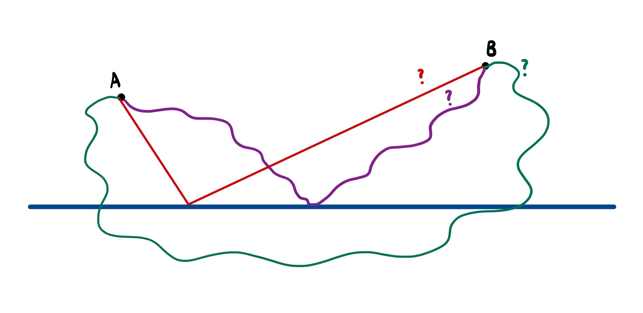
We begin with a classic problem before delving into more niche use-cases: Heron’s shortest path problem. In this, we consider two villages, A and B, on the same side of a perfectly straight river. We wish to find the shortest path from village A to B that touches the river at some point.
Calculus provides a robust but rather inelegant solution to this problem. First, we define the following variables:
- $a$, $b$: the perpendicular distance from village A, B to the river, respectively
- $x$: the length along the river that we touch it at
- $l$: the distance along the river between village A and B
These are illustrated in the following diagram.
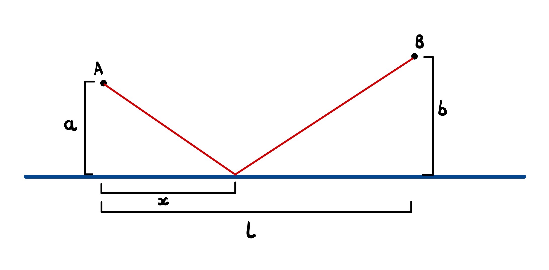
Using Pythagoras’s theorem, we can see that the total length of the route is
$$L(x) = \sqrt{a^2 + x^2} + \sqrt{(l - x)^2 + b^2}$$
We can then differentiate this once to find any turning points and once again to confirm we have a minimum. It’s a safe approach, but as we’ll see, it’s a lot more work than is needed.
Instead, we can apply the reflection principle by making a clever observation: any path from A to B touching the river can be associated with a path of the same length starting from the reflection of A (we’ll call this A’) in the river to B. This is best seen in the following diagram.
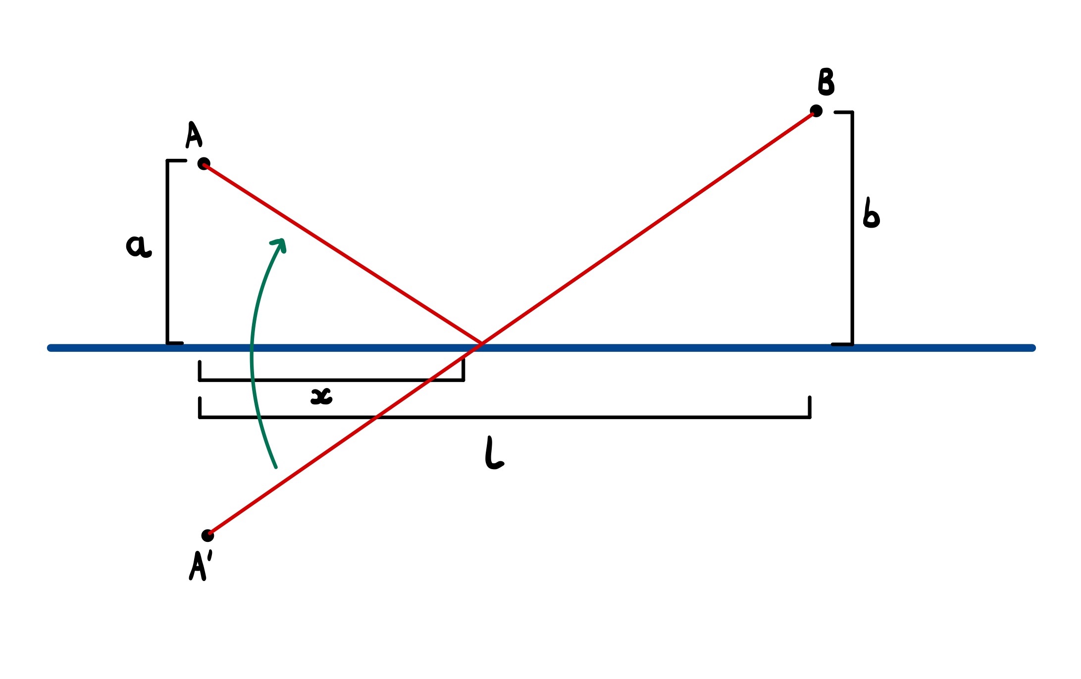
This tells us that our initial problem is equivalent to finding the shortest path from A’ to B that touches the river. But here’s the kicker: every path from A’ to B must pass through the river (as they’re on different sides of it). We’ve therefore reduced our problem to finding the shortest path between two points subject to no extra conditions—i.e. a straight line. We can then reflect the part of the path below the river to retrieve the solution to our original problem.
This immediately tells us that the shortest path has a length of $\sqrt{l^2 + (a + b)^2}$ (Pythagoras) and the optimal crossing point is $\frac{al}{a + b}$ down the river from A (similar triangles). No calculus, no root finding. Simple.
Bouncy Random Walks
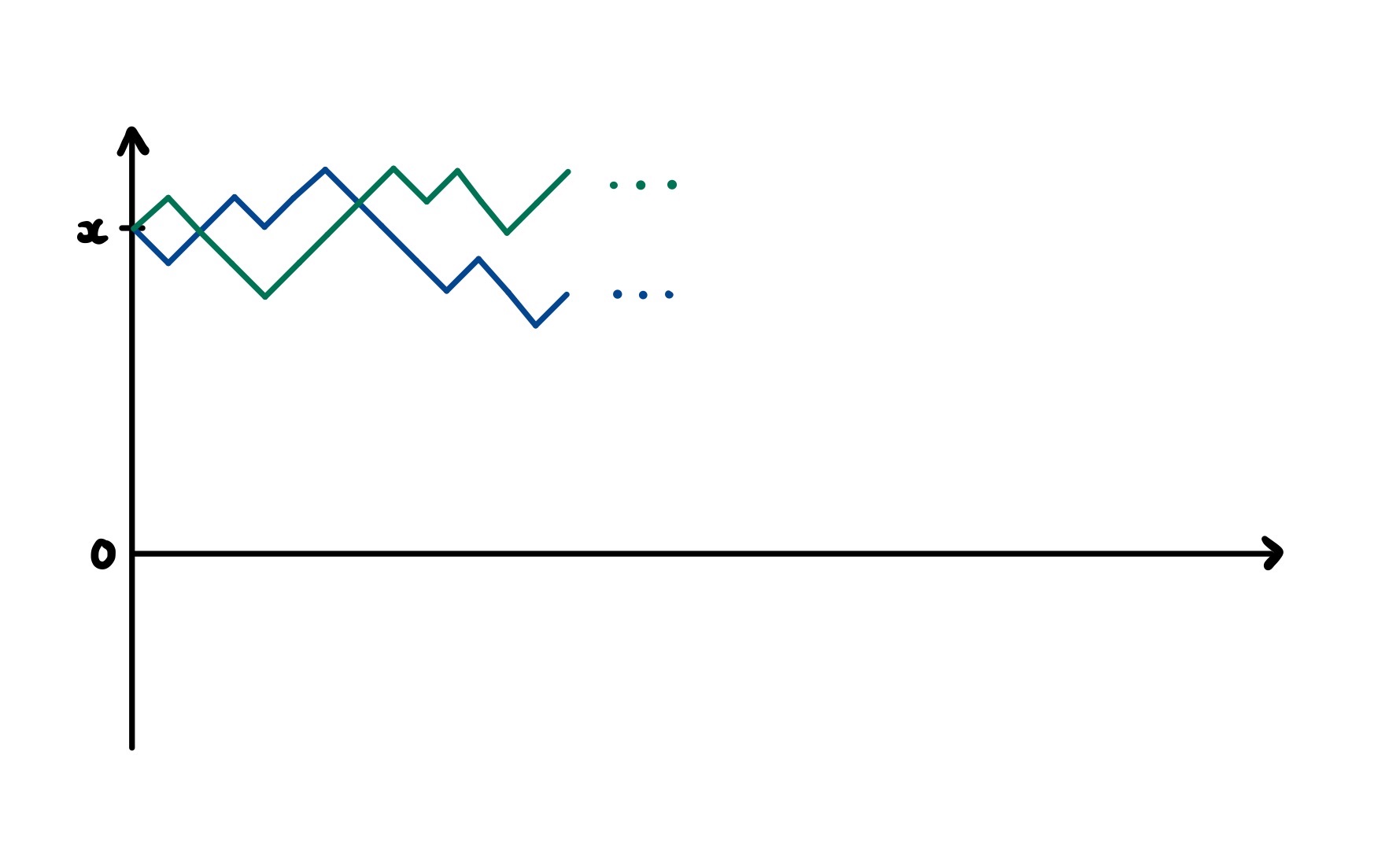
We now move on to a related problem is quantitative finance. In this, we model the movement of a stock’s share price as a discrete-time random walk on the integers starting from £$x$. That is, we start at time $t = 0$ with a share price of £$x$ and at each time step this either increases by £1 with probability $p$ and decreases by the same amount with probability $1-p$. Two examples of such a random walk is shown below. For simplicity, we allow the share price to go into negatives.
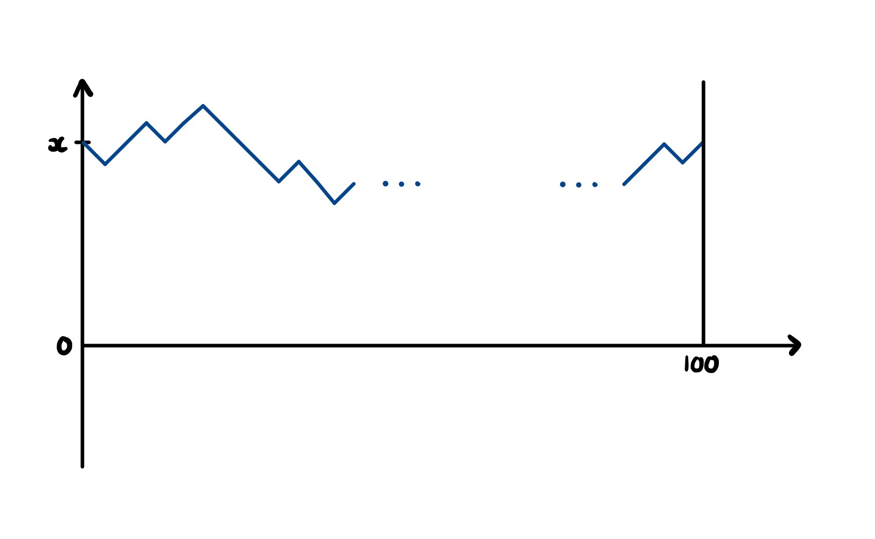
We start by asking what is the probability that our stock will have returned to the initial price £$x$ at time $t = 100$. This problem isn’t too difficult to answer using the binomial distribution. We can think of the price movement up to time $t = 100$ as a series of coin flips using a biased coin (probability $p$ of getting heads). Our final share price will be the initial price plus the number of heads and minus the number of tails.
If we want the final price to be the same as the initial, we require an equal number of heads and tails ($50$ each). In other words, we just want to know $\mathbb{P}(X = 50)$ where $X \sim \textrm{Binomial}(100, p)$. This is simply
$${100\choose 50}p^{50}(1-p)^{50}$$
It is not too difficult to generalise this to any final time or share price (as we’ll see below). What isn’t immediately obvious, however, is how we can find the above probability if we also stipulate that the stock price must hit £$0$ at some point before returning to £$x$ at time $t = 100$. Passing through zero sounds an awful lot like crossing the river in the previous problem—it seems like the reflection principle will be of use again.
Indeed, just as before, we can build a correspondence between all stock paths from $x$ to $x$ that hit $0$ with all unrestricted paths from $-x$ to $x$. This means that we no longer have to worry about whether our paths hit $0$—since they cross from negative share prices to positive in steps of size one, they all have to.

We are simply left to calculate how many paths there are from $-x$ to $x$. Using the same binomial approach as before, we have $100$ coin flips, but this time we need there to be $2x$ more heads than tails. To avoid overcomplicating things, let’s say that $x=10$. In this case, we need $60$ heads and $40$ tails, occurring with probability
$${100\choose 60}p^{60}(1-p)^{40}$$
Note that this is smaller than the probability above, which makes sense given that we added a restriction to the paths we are considering.
Laser Beams
The final puzzle I want to discuss is, in fact, the main inspiration for writing this blog post. It is an example of a rather fiendish-looking puzzle that reveals a beautifully simplistic core when approached with the right technique. It involves firing a laser beam into the reflective interior of an equilateral triangle, with infinitesimal gaps at the vertices. For any integer $n$ we want to know how many angles we can fire the laser at, such that the beam will leave through the same hole it entered after exactly $n$ bounces.
At first glance, this problem seems monstrous. Computing the angle and contact points of the laser beam becomes increasingly difficult as more bounces occur, quickly becoming intractable.
By looking back at the previous two examples, let’s try to summarise exactly what the reflection principle involves, so we can see how it could apply to this problem. Specifically, in both cases we started with a problem in which we required our path to be reflected. This proved conceptually difficult, so we tried a different approach—reflecting the world around our path.
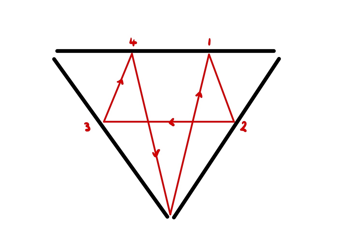
In the first example, our reflected line became a straight line starting from a reflected village. Likewise, in the second, our reflected path became an unrestricted path starting from a reflection of the initial share price. A similar idea can be used for this problem: rather than reflecting the laser beam’s path, we pretend it has a perfectly straight trajectory and reflect the world around it instead. That is, whenever the laser hits a mirror, we let it continue on its original path and create a reflected copy of the triangle on the other side of the mirror. This is illustrated the following diagram, which shows a single laser beam path visualised in two ways.
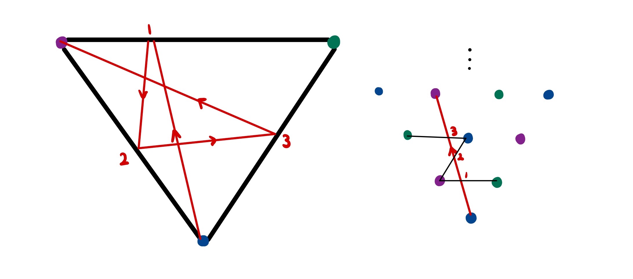
It may not be immediately obviously how much of a simplification this perspective change has made to our problem. To see this, let’s make a few observations.
First, we no longer have to worry about defining a laser beam’s path by the angle it enters the triangle at. Instead, we can create a coordinate system for the expanded triangular grid and relate each angle to the coordinate of the vertex it is pointed at. We can extend this even further by noting that if we point at vertex $(4, 6)$, we will hit vertex $(2, 3)$ first. In other words, it is only possible to reach a vertex whose coordinates are coprime. It is also easy to tell what vertex the beam will leave the triangle at given this target coordinate since the vertex colours have a consistent pattern.
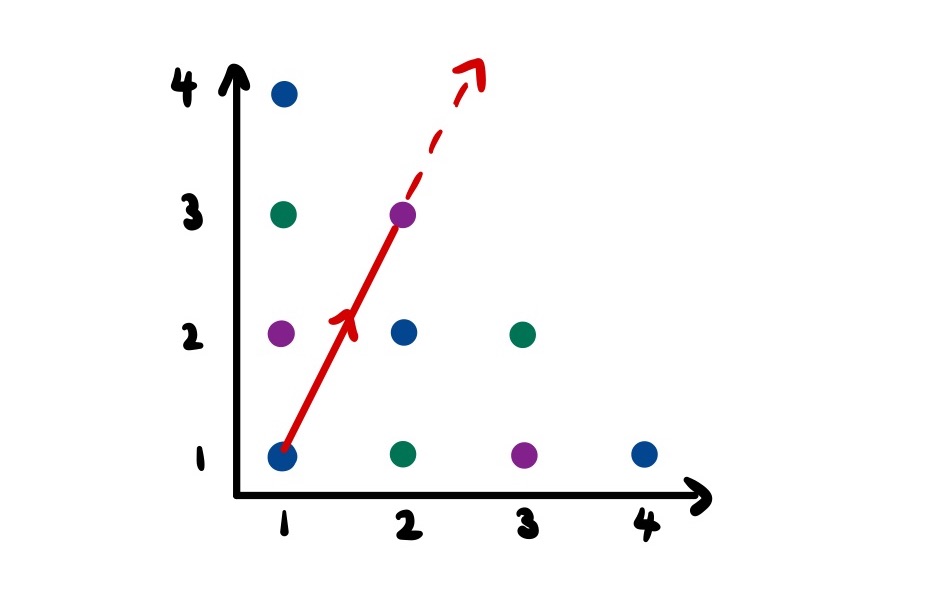
Second, it is easy to see in this representation how many bounces a laser beam angle (defined by a coprime pair of coordinates) will result in. Specifically, reaching a new level of the grid requires crossing two lines which correspond to reflections.
Combining these two facts, we see that our previously intimidating problem has been reduced to finding coprime numbers that sum to a given target. I have to be deliberately vague about the details and implementation of this procedure since it relates to a Project Euler question that I do not wish to spoil. Never-the-less, this simplification has taken us the majority of the way to the solution, hopefully driving home how useful the reflection principle can be.
If you have other applications of the technique, I would encourage you to share them below.