
The Setup
Suppose we have a fixed amount of money that we have set aside for investment. We have narrowed down the equities we to a list of length $n$. From analysing historical data we know the vector of expected returns for each equity $v$ and the covariance matrix of returns $\Sigma$..With that in mind, our goal is to choose the simplex vector $x$ (i.e. $0\leq x_i \leq 1$, $\sum x_i = 1$) that maximises our expected return for any given risk tolerance $r=x^T \Sigma x$.
If we were to find this $w$ for each $r>0$ and use this to calculate our expected return $e = v^T x$, we would end up with a curve known as the efficient frontier, which maximises our return for any given risk tolerance.
I became aware of the efficient frontier when talking to a collegue about a project he was working on. As an intermediate step, this involved calculating efficient frontiers, and I was surprised to see the approach that he was taking. It involved randomly generating a large number of simplex vectors, calculating their associated risk and expected return, before plotting these all on a graph as shown below.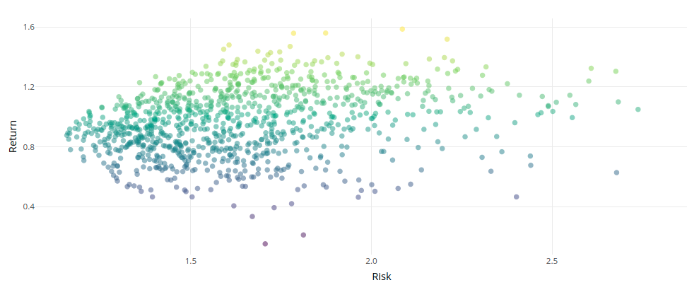
With enough simulations, you become able to see the outline of the efficient frontier, the curve marking the top boundary of the data points. This could then be turned into a curve by calculating the convex hull of the points, perhaps with some added smoothing.
This approach stood out to me for two reasons:
- There was no way it would scale; as the number of equities increases, the space of portfolios to explore grows roughly exponentially. This means that the solution is not appropriate for real-world use where you would wish to consider a large number of equities.
- The efficient frontiers generated looked an awful lot like a parabola—if this was the case then surely there was an analytic way of finding the equation of this curve.
Another popular approach for computing the effient frontier is using gradient descent. Under the right assumptions (the same as we will introduce later), the problem we are looking at is convex, and so we are guaranteed to find a local optimum, with convergence that is quadratically fast. This is still slower than the method we’ll look at below so we won’t discuss it further, but it is worth noting that it is also much more efficient than the random approach above.
An Analytic Approach
As mentioned above, I was immediately suspicious that an analytic solution existed to the efficient frontier problem. It turned out that this was the case provided we introduced one key assumption: shorting is valid. I will not get into the financial definiton of short-selling now (though you can read about here). All we need to care about is that it corresponds to use removing the bounds on our portfolio weights $x_i$. We still however enforce that $\sum x_i = 1$. Under this condition, our problem becauses a quadratic programming problem which can be solved using Lagrangian multipliers. Note, it is algebraically more elegant to solve the dual form of our problem (minimise risk for a given return), though the same solution is arrived at.
It is worth noting that although the introduction of shorting might make this analytic solution inappropriate for markets that do not allow it (more discussion on this later), the opposite flaw exists for the randomised approach we saw earlier in that it only works when shorting is forbidden, else the space of solutions to explore grows to intractable proportions.
Our problem can be stated as
$$
\begin{align}
\text{minimise} \quad & w = x^T \Sigma x \\
\text{s.t.} \quad & v^T x = e \\
& 1^T x = 1
\end{align}
$$
The corresponding Lagrangian is
$$\mathcal{L}(x, \lambda, \mu) = x^T \Sigma x - \lambda (v^T - e) - \mu (1^Tx - 1)$$
The derivative is therefore
$$\Delta_{x, \lambda, \mu}(x, \lambda, \mu) = \begin{pmatrix}
2x^T\Sigma - \lambda v^T - \mu 1^T \ e - v^T x \ 1 - 1^Tx
\end{pmatrix}$$
Note, that this is a vector of length $n+2$. The usual way to proceed would be to set this equal to zero and solve the resulting system of equations through substitution. I tried this for a while and stuggled greatly. This is when I noticed a clever cheat which draws the straight out. This was to write the above system as a matrix equation in $x$, $\lambda$ and $\mu$.
$$
\begin{pmatrix}
2\Sigma & v & 1 \\
v^T & 0 & 0 \\
1^T & 0 & 0
\end{pmatrix}
\begin{pmatrix}
x \ \lambda \ \mu
\end{pmatrix}
=
\begin{pmatrix}
0 \ e \ 1
\end{pmatrix}
$$
It is easy to verify that the matrix on the left is invertible whenever $\Sigma$ is postive definite (a reasonable assumption). To do this we use the following expression for the determinant of a block matrix.
$$
\text{det}
\begin{pmatrix}
A & B \\
C & D
\end{pmatrix}
= \text{det}(A) \cdot \text{det}(D - CA^{-1}B)
$$
Alternatively, you can solve for $x$ directly, to avoid the extra cost of solving the entire system.
Try It For Yourself
Since the matrix above is symmetric, postive definite, we can use efficient methods for solving the system. This gives us the optimal value of $x$ with incredible efficiency. To illustrate this difference, I have developed a Shiny dashboard to demo the initial and efficient approaches, benchmarking there runtimes to show how vastly superior this approach is. You can find the dashboard here.
Wrapping Up
Two final thoughts…
How much does the optimal portfolio under shorting differ from that without? Could we simply project the shorted solution onto the space of non-shorted solutions to obtain an approximately optimum solution. I hope to return to this problem at a later point, hoping to obtain either exact or probabilistic bounds.
After discussing this project with another collegue, it turns out that this solution is not completely original (though I believe my method of proof is novel and more elegant than other approaches). That said, it was original to me at the time of discovering this approach, which I think is good enough for an undergraduate.