
The Excel spreadsheet used in this post can be found on the GitHub repository for this blog
Formulating the Coverage Problem
Suppose that you work at a telecommunications company and one day you are sent an Excel spreadsheet with the following data.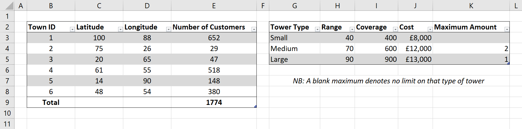
As you can see, the data concerns the location of 6 towns and the number of customers the company has at each one. You are informed that the company wishes to build new communication towers in a selection of these towns so that every customer is covered by at least one tower (we assume that currently no town has any existing coverage). Your objective is to determine the cheapest way in which this can be achieved. The data goes on to detail that there are three sizes of tower available to be built, each with its own associated range, coverage (that is the number of customers it can sustain), and construction costs (we assume that running costs are negligible). There are also limitations on the number of some of the types of satellite you can build. A further constraint is that due to planning permission issues, you can only build one tower in any given town. Lastly it is added that if two towers cover the same customer then only one of them needs to use its coverage to serve that customer.
This feels very close to the sort of problem a real life telecommunications company may be trying to solve albeit with reduced scale and complexity. The expanse of this example is not limited by the methods we will be using but rather the tool - Microsoft Excel. Using a more powerful method such as a programming language like Python or Matlab would facilitate the expansion of this problem further. Despite this, I believe that this example captures the essence of the problem with the added bonus that it can be formulated in a visual way in a spreadsheet.
We will solve this problem using linear programming; in particular, the branch and bound algorithm. To do this we will need to build a model to describe the problem and then use the Solver add-in in Excel to find an optimal solution. Before we get to this, let’s take a look at this problem through a mathematical lens.
A Mathematical Description
We begin by formulating the problem mathematically. If you are only interested in the practical side of this problem then feel free to skip this section but I would argue that any good Excel model will have a well-thought-out mathematical model behind it.
Decision variables
To begin, we will need to define a collection of decision variables. For shorthand, we denote the towers sizes small, medium, and large by the integers 1, 2, and 3 respectively.
$$
c_{i,j} :=
\begin{cases}
1 & \textrm{if town } j \text{ is covered by a tower in town } i \\
0 & \textrm{otherwise}
\end{cases}
\qquad
i \in[6], j \in [6]
$$
$$
n_{i,j} :=
\begin{matrix}
\textrm{the number of customers in town } \\
j \textrm{ covered by a tower in town }
\end{matrix}
\qquad
i \in[6], j \in [6]
$$
$$
t_{i,k} :=
\begin{cases}
1 & \textrm{if a tower of size } k \text{ is built in town } i \\
0 & \textrm{otherwise}
\end{cases}
\qquad
i \in[6], k \in [3]
$$
The first two sets of variables may seem redundant when put together but we do in fact need both of these. The use of the second is clear but the first is more subtle. This is used when checking whether the tower range criterion has been met. We want town $i$ to be in the range of town $j$ whenever at least one customer in town $j$ is being covered by a tower in town $i$, otherwise we have no restriction. This condition can be described using an if statement on the expression $n_{i,j} \geq 1$ but such conditional expressions are non-linear so instead we have to use a new decision variable to represent this and force it to behave in the desired way using additional constraints. This will be explained in more detail shortly.
Constants
We will also need a way of describing the data we are given at the beginning of the post. We denote the latitude and longitude of town $i$ by $\textrm{lat}_i$ and $\textrm{long}_i$ although these are not very useful to us so we immediately replace them with the 6x6 matrix $D = (d_{i,j})$ with the $(i,j)$th entry representing the Euclidean distance between towns $i$ and $j$. That is
$$d_{i,j} := \sqrt{(\textrm{lat}_i-\textrm{lat}_j)^2 + (\textrm{long}_i-\textrm{long}_j)^2}
\qquad
i \in[6], j \in [6]$$
We also define a 6-element column vector $\hat{\nu} = (\nu_i)$ where $\nu_i$ is the number of customers in town $i$, as well as 3-element column vectors $\hat{\rho} = (\rho_k)$, $\hat{\gamma} = (\gamma_k)$, $\hat{\pi} = (\pi_k)$, and $\hat{\mu} = (\mu_k)$ where $\rho_k$, $\gamma_k$, $\pi_k$, and $\mu_k$ represent the range ($+\infty$ if not specified), coverage, cost (price), and maximum number allowed for each tower respectively.
Objective function and constraints
Our objective function is simple; we just wish to minimise costs. In mathematical language, this is
$$\textrm{min } w = \sum_{k=1}^3 \left(\pi_k \sum_{i=1}^6 t_{i,j}\right)$$
We can now begin to formulate our constraints. We start with the simplest; that is the limit on the number of towers in each town and towers of each type. These are formulated as
$$
\sum_{i=1}^6 t_{i,k} \leq \mu_j \qquad \forall k \in [3] \tag{1}
$$
and
$$
\sum_{k=1}^3 t_{i,k} \leq 1 \qquad \forall i \in [6] \tag{2}
$$
We can now add the constraint that every customer must be covered by at least one tower. Since the customers are indistinguishable, we only require that the potential coverage for each town is larger than the size of the customer base there. That is
$$
\sum_{i=1}^6 n_{i,j} \geq \nu_j \qquad \forall j \in [6] \tag{3}
$$
Similarly, we also need that the total coverage provided by any town is at most the maximum coverage that its tower can supply. Since every town can have at most one tower we have that the maximum coverage is just $\sum_{k=1}^3 \gamma_k t_{i, k}$ (which is zero if no tower is built in that town, as expected) and so we can write
$$
\sum_{j=1}^6 n_{i,j} \leq \sum_{k=1}^3 \gamma_k t_{i, k} \qquad \forall i \in [6] \tag{4}
$$
Now is an appropriate moment to add a constraint to link the behaviour of each $c_{i,j}$ and $n_{i,j}$. We require that $n_{i,j}$ is zero whenever $c_{i,j}$ is zero, and have no restriction when $c_{i,j} = 1$. Some might say that we should force $n_{i,j}$ to be strictly positive if $c_{i,j} = 1$ but this is redundant since the model will force this behaviour naturally - it would be sub-optimal to cover a new town, possibly worsening the range constraint and then not serve any customers there. We first define $M = \sum_{i=1}^6 \nu_i$ to be a large constant representing the total number of customers across all towns. Then, we use the following constraint to link the variables
$$n_{i,j}\leq Mc_{i,j} \qquad \forall i \in [6], j \in [6] \tag{5}$$
Lastly, we need a constraint to control the ranges of the satellites. This is the most complicated to implement but using the variables $c_{i,j}$, it becomes reasonably simple
$$d_{i,j}c_{i,j} \leq \sum_{k=1}^3 t_{i,k} \rho_ \qquad \forall i \in [6], j \in [6] \tag{6}$$
Note that since $j$ does not appear on the left-hand side, this can be rephrased as
$$\max\limits_{j\in[6]}( d_{i,j}c_{i,j}) \leq \sum_{k=1}^3 t_{i,k} \rho_ \qquad \forall i \in [6]$$
Though this is no longer linear.
This concludes the constraints for the problem and so the entire linear programming formulation too. In total we have 90 decision variables and 93 constraints, plus the implicit constraints that 54 decision variables and binary and the other 36 are non-negative. If we generalised this problem to have $n$ towns and $m$ towers, a similar calculation gives $n(m+2n)$ decision variables and $m+3n+2n^2$, with the implicit constraints that we have $n(m+n)$ binary variables and $n^2$ non-negative real variables. It is clear that this problem will become computationally infeasible very quickly as both variables are increased.
We are now in a strong position to begin translating these mathematical relations into an Excel model.
Modelling the problem with Excel
The distance matrix
For clarity in Excel formulae, I began by assigning names to the two tables in the data sheet. I named the left table TownData and the right table TowerData. Then, the first step in building our Excel model is to convert the Cartesian locations of the towns into a distance matrix. I did this by adding a new sheet in the workbook named ‘Distance Matrix’ and creating a table to contain the distances. This is the final result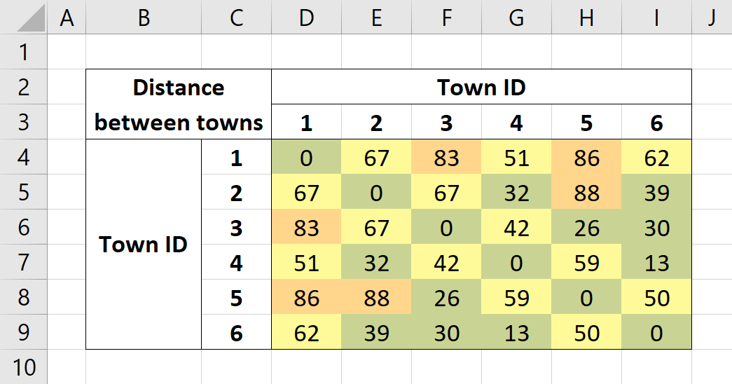
The values in the table are generated by several VLOOKUP formulae. In particular, for cell D4 I used
1 | =SQRT((VLOOKUP(D$3, TownData, 2) - VLOOKUP($C4, TownData, 2))^2 + |
Breaking this down, the first VLOOKUP statement, VLOOKUP(D$2, TownData, 2), looks in the TownData table and finds the row matching matching the value in D3, the label of the column we are in, and then selects the second column (latitude) from that row of the table. The other 3 VLOOKUPs are similar. C4 is used to select the label of the row that we are in and we replace the third argument with 3 to select the third column of TownData, longitude. I then used the standard formula for the Euclidean distance between two points to give the final value. Note, that I anchor the row for D3 and the column for C4 using the dollar symbol so that when this formula is copied to the other cells in the table, the row and column labels are referenced correctly.
I then applied some formatting to the table. Firstly, I changed the data type for the inner cells to have no decimal places displayed to improve clarity. I then applied a series of conditional formatting rules to the table to colour the cells green, yellow, orange, or red depending on whether the distance between any two towns could be covered by every tower, the two largest towers, just the largest tower, or none. This makes the assumption that the ranges of the towers are increasing with size which will almost certainly be true in reality and so if our input data is valid, we will not have any issues here. In this example we have no red cells but if we change the range of the largest tower to be 80 we get the following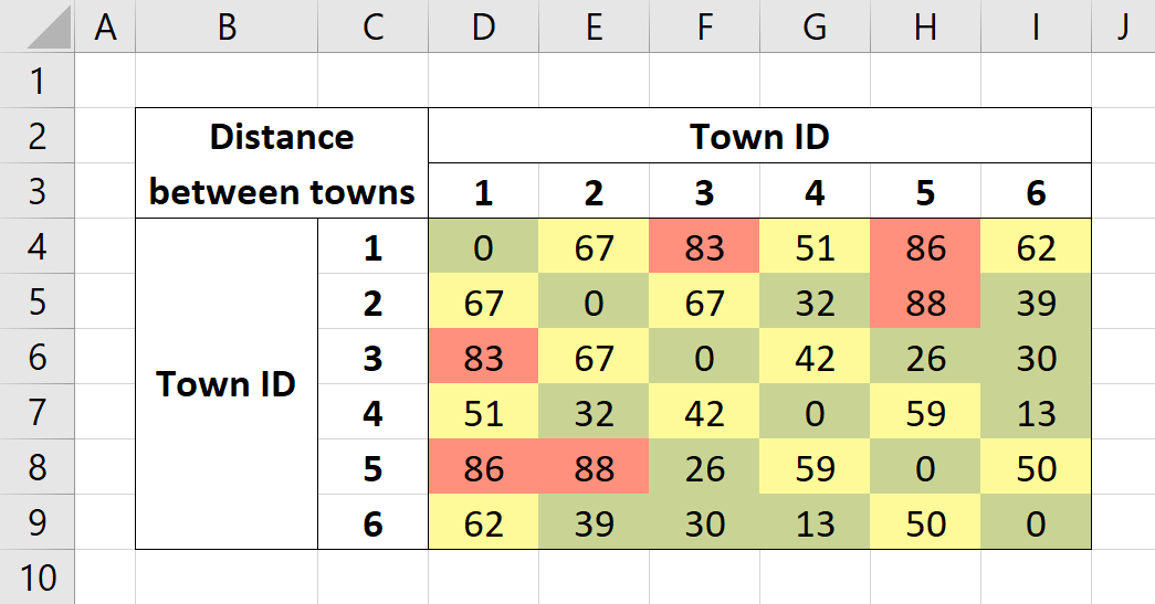
The full model
We are now ready to begin building the full model. I decided to do this on another separate worksheet using the following layout. As mentioned at the start of the post, the final Excel spreadsheet can be found on the GitHub repository for this blog.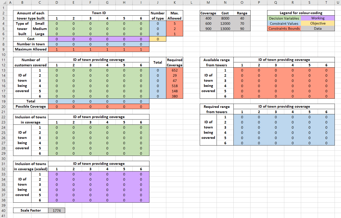
This may seem daunting at first glance but when it has been broken down to its constituent parts, it is much more palitable. As can be seen in the key, the green cells represent decision variables. For those that read the mathematical formulation, the upper set correspond to $t_{i,k}$, the middle set to $n_{i,j}$, and the lower set $c_{i,j}$. For the time being these are filled with zeros, acting as place-holders. We also have a small grey table at the top and a lone grey cell at the bottom. Their purposes will be discussed later but all that needs to be known for now is that they are constructed by using VLOOKUP statements to copy values across from the data worksheet.
Let us now look in more detail at the top-left table (cells B2:K9). The blue cells on the right are calculated by summing the rows of the inner table and so represent the total number of each tower type built. This is compared to the maximum number of each tower allowed in the red cells next to them. These values are taken directly from the data worksheet using a VLOOKUP statement, although observe that since our lookup value is a string we need to set the optional range_lookup parameter to be FALSE else we get erratic behaviour. These values are then passed into IF statements to handle the case when they are a blank string. In this case we are allowed an unlimited amount of that type of tower. We cannot represent infinity in Excel so instead we set it to the ceiling of total number of customers divided by the maximum coverage of that tower type since we would never need more towers than that for a reaistic problem. An alternative approach would be to set this to 6 since we only have that many towns, each of which with one possible tower but using the former method generally produces a tighter formulation of the problem and so improve runtime. For a specific example, the formula for cell K4 is
1 | =IF(ISBLANK(VLOOKUP($C4, TowerData, 5, FALSE)), |
The purple row below the inner table simply uses SUMPRODUCT with the column above and the costs of each tower to calculate the build cost for each town. These are then summed up in the gold cell to give the total cost (our objective function). The blue row below this is simply a sum of the inner columns above and so represents the number of towers in each town. This is compared to the fixed value of 1 in each case.
The setup for the table below this (B11:K20) is very similar We sum the rows and columns as before to get the blue cells. The row sums represent the number of customers that can be covered in each town and the column sums represent how many customer a tower in a given town is covering. On the right we then compare these to the size of the customer base in each town taken from the data worksheet using another VLOOKUP statement. On the bottom we compare these to the range of the chosen tower (or lack of) by computing the SUMPRODUCT of the corresponding column of the inner upper table and the coverage data for each tower. For example, the formula in D20 is =SUMPRODUCT(D$4:D$6, $M$3:$M$5).
The model now gets slightly more convoluted due to the limitations of the two dimensions of a spreadsheet. Since Excel Solver constraints cannot handle additional constants, we must manually multiple our coverage decision variables ($c_{i,j}$) by our large constant ($M$) We do this using the array formula {=$D$40 * $D$24:$I$29} applied to the cells D33:I38. We will later use these new scaled variables to control the behaviour to control the behaviour of the middle table of decision variables ($n_{i,j}$).
Lastly I add two tables on the right to apply the range contraints. The lower green table is simply the product of the distance matrix and the coverage decision variables ($c_{i,j}$) in the lower green table using an array formula. This represents the range required for any particular tower covering some town. These will later be compared to the red table above. Each column in the inner table contains the exact same formula which computes the SUMPRODUCT of the corrsponding column of the top-right inner table and the range data. For example, all of the cells O13:O18 contain =SUMPRODUCT(D$4:D$6, $O$3:$O$5).
With some additional static formatting, I achieved the result shown above. In particular, I set the data type for each numeric cell to be integral. This is because our problem is complex enough that Excel Solver will only return an answer to a given tolerance rather than an exact solution. However, we are only interested in the exact solution and these will be close enough to this that it will be okay to round. The next step is to setup the Solver add-on and find an optimal solution to the problem.
Finding an optimal solution
If you wish to reproduce this example, it is import to make sure that you do in fact have the Excel Solver add-in enabled. If this is not the case, you can learn how to do this through this support document.
I setup Solver as follows
Some of the parameters are standard. Our objective cell is J7 and we wish to minimise this. Our decision variables are all of the green cells, that is D13:I18, D4:I6, and D24:I29. We also wish to make D4:I6 and D24:I29 binary variables and so two of our parameters control this. The other variables we need to be non-negative and so we select ‘Make Unconstrained Variables Non-Negative’. Our problem is linear so we use the Simplex engine.
We can now take a look at the other constraints we added. The first is that D13:I18 should be element-wise less than or equal to D33:I38. This corresponds to constraint 5 in the mathematical formulation and is used to force the number of customers in town $j$ covered by a tower in town $i$ to be zero whenever the tower in town $i$ is not covering town $j$ and unrestricted otherwise.
The next constraint says that D19:I19 must be at most D20:I20 for each element. This corresponds to the constraint that the number of customers covered by a tower in town $i$ can be at most the available coverage (or lack of) of the tower in that town. This relates to constraint 4 above.
We then have the two binary constraints which we have already discussed.
The next constraint limits the elements of D8:I8 by the corresponding elements of D9:I9 which take a constant value of 1. This refers to the constraint that only one tower can be built in each town. This is constraint 2 in the mathematical formulation.
We then have a constraint that the values of J13:J18 must be element-wise greater than or equal to K13:K18. This relates to the requirement that every customer is covered by at least one satellite. This is constraint 3 from the last section.
The penultemate constraint says that J4:J6 can be at most the value of K4:K6 for each element. This simply represents that you cannot build more towers of one type than the given maximum, the first constraint from above.
The final constraint says that each element of O22:T27 must be less than or equal to O13:T18. This is used to ensure that no tower covers a town outside of its range. This is constaint 6 in the mathematical formulation.
This concludes the setup for this problem. Clicking ‘Solve’ begins the branch-and-bound Simplex algorithm and after a few seconds (and around 800 sub-problems) we get the optimal solution shown below (within a negligable tolerance).
Reading of the decision variable, we see that the (although there may be more) optimal solution is to build a small tower in town 2, a medium tower in town 1, and a large tower in town 4. We use the medium tower in town 1 to cover 571 customers in itself and, interestingly, all 29 customers in town 2. The small tower in town 2 is then used to solely cover town 6 with spare coverage for 20 customers. The large tower in town 4 is then used to covered all other customers exactly in towns 1, 3, 4, and 5. The cost of this coverage is £33,000.
Due to the nature of this problem, there will obviously be many different equally-optimal solutions with different exact coverages for each town pair. This blog post is already very long but if I were to continue, I would next fix the optimal price and choose a second objective to function to optimise whilst maintaining the total cost to find a more practical optimal solution. For example, I may try to optimise the amount of overall spare coverage to future proof the network, or attempt to spread the spare coverage around more evenly by adding some padding to the coverage constraints. Another idea might be to add bias to make coverage of closer towns more favourable, although this would require some careful formulation.
I encourage any reader to download the spreadsheet form the GitHub repository for the blog and try using this model with your own data. The model can be customised by adding or removing rows and columns to change the number of towers and towers. It is worth noting however that the scale and complexity of this problem is right on the edge of the default Excel Solver’s limitations. The add-in allows for up to 200 decision variables of which we are using only 90, however our real issue is the constraint limitation of 100, leaving us with only 7 spare. Even with the current setup, for unusual inputted data, the model can take several minutes to return and optimal solution, running through thousands of sub-problems in the process. In some pathologiacal cases I have discovered, this can be up to tens of minutes. These examples are often not very realistic as they involve towns that are no longer homogenously distributed but instead put deliberately far away form each other. Furthermore, without any limits on the number of each type of tower, the problem can take a long time to solve as the solution space is much larger.
To overcome these problems there are two solutions. The first is to use a propriety Solver add-in for Excel such Frontline Solvers. This product is made for large coparations some comes with a a heafty price-tag in the thousands of dollars however it is much faster than the standard add-in and can support up to 2000 decision varibales and 8000 constraints for linear problems. My much more prefered solution however is to use a linear programming library for an open-source programming language such as scipy.optimize for Python or JuliaOpt for Julia. I would avoid using R, although some good linear programming packages do exist, due to its reduced numerical computation speed. If you have access to propriety mathematical languages such as MatLab and Mathematica, these also have very powerful optimisation libraries capable of solving linear programming problems like this in much faster times and with greater scale than Excel Solver. Despite this, for a simple, explainable, and visual model of modest size, Excel really can’t be beat.